Global Liquidity Explained: Why Liquidity Matters for Stocks, Crypto and Market Cycles

Executive Summary

Global liquidity describes the availability of money, credit, and financing capacity across the financial system, and it is, in my view, one of the most important variables for understanding where markets are in their cycle. There is no single perfect measure of it. E.R.A. OF CHANGES evaluates several components together: major central-bank balance sheets, bank reserves, the Federal Reserve’s reverse repo facility, Treasury cash management, broad money supply, private credit conditions, and cross-border dollar funding. Each captures a different dimension of how much capital the financial system can deploy and at what cost.

Liquidity expansion can support valuation multiples, risk appetite, and the ability to carry leverage, even when economic fundamentals have not yet visibly improved. Liquidity contraction can produce deleveraging and multiple compression even when corporate earnings initially remain intact. Crypto and other high-beta assets have shown particularly strong sensitivity to liquidity and leverage conditions, though that relationship is not mechanical and has become more complex with institutional adoption.

Fiscal policy can partially offset monetary tightening, which means simple Fed-balance-sheet narratives often give an incomplete picture of the system. The most useful approach is to identify changes in the liquidity regime and confirm them through credit spreads, funding conditions, and market behavior rather than trading a single data series in isolation.

Key Takeaways

• Global liquidity is a system of related variables, not one statistic. No single measure captures the full picture.
• E.R.A. OF CHANGES places particularly high importance on liquidity when identifying the underlying market regime, especially for the six-month outlook.
• Central-bank balance sheets matter, but bank reserves, the Fed’s reverse repo facility, Treasury cash balances, and private credit conditions can materially change the interpretation.
• M2 is an important liquidity filter but does not capture every form of market funding, cross-border financing, or central-bank operation.
• Expanding liquidity can support higher valuation multiples and greater risk appetite even before economic fundamentals improve.
• Contracting liquidity can force deleveraging even when corporate revenue initially remains strong.
• Crypto tends to exhibit high sensitivity to liquidity and leverage conditions, but the relationship is not a deterministic pricing model.
• Fiscal policy can partially offset monetary tightening, which is why “Fed tightens = markets tighten” has repeatedly failed as a complete framework.
• Cross-border dollar funding becomes critical during periods of global stress.
• Liquidity signals should be confirmed with credit spreads, funding conditions, and market structure before drawing conclusions.

Introduction

Here is a contradiction that has puzzled retail investors for decades. Equity markets can rally strongly while economic data looks mediocre. Earnings estimates can be revised downward while stock prices still make new highs. And conversely, markets can fall sharply even while corporate profits remain healthy and GDP growth is positive. The explanation, in many cases, is not found in the economic statistics. It is found in what is happening to the financial system’s capacity to deploy capital.

Fundamentals influence the long-term value of an asset. Liquidity strongly influences the financial conditions under which that value gets priced on any given day, month, or year. Discount rates move with liquidity. Leverage capacity moves with liquidity. The marginal buyer’s willingness to take risk moves with liquidity. These are the variables that determine whether the market is willing to pay 20 times earnings or 14 times earnings for the same business at the same moment in its cycle.

The question this article answers is what global liquidity actually is, how investors should think about measuring it, and why it matters so much for equities, crypto, credit, gold, and the broader market cycle.

What Is Global Liquidity?

Global liquidity refers to the availability of money, credit, and financing that can support economic activity, asset purchases, leverage, and cross-border capital flows. It includes both official liquidity (created or influenced by central banks, government cash management, and monetary facilities) and private liquidity, created through commercial banks, capital markets, shadow banking, and cross-border financing.

The important distinction is this: global liquidity is considerably broader than the amount of money central banks have printed. A central bank can expand its balance sheet and find that the additional reserves remain largely idle within the banking system, while private credit creation is contracting simultaneously. The net liquidity available to the real economy and to financial markets is the combination of both channels, minus what is being absorbed by government financing, regulatory requirements, or institutional cash management.

Why There Is No Single Global Liquidity Number

This point is where a lot of popular analysis goes wrong, and I want to be direct about it. Different measures capture genuinely different things.

The Federal Reserve’s consolidated assets were approximately $6.748 trillion on September 23, 2026. That balance sheet measures the central bank’s asset holdings; it does not by itself tell you how funding is reaching borrowers. U.S. seasonally adjusted M2 was $23.3428 trillion in August 2026 in the September 22 H.6 release. M2 measures currency and selected deposit and retail money-market-fund balances within the United States, not total credit or a global pool of investable cash. Source. Source 2.

U.S. M2 does not include the ECB, the Bank of Japan, private credit in emerging markets, or cross-border dollar funding. Reserve balances held by depository institutions at Federal Reserve Banks averaged approximately $2.93 trillion in the week ended September 23, 2026; the Wednesday observation was approximately $2.97 trillion. These are different observations of the same defined reserve-balance series. Reserves matter for funding conditions, but their aggregate level is not by itself a measure of credit availability to borrowers. Source.

Each of these series is useful. None of them is the whole picture.

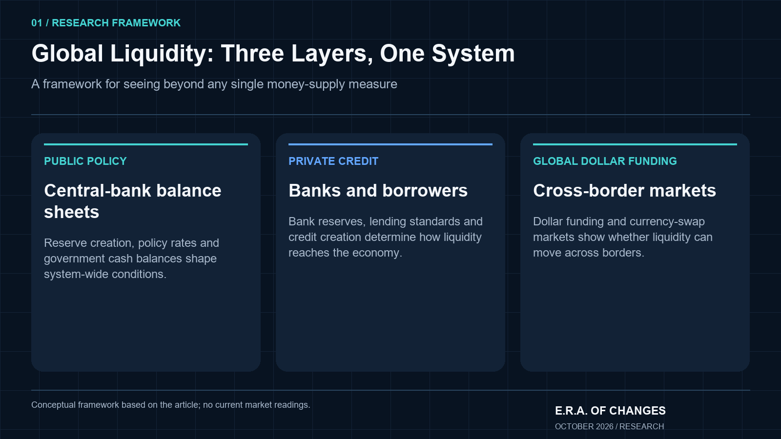
Our Seven-Component Global Liquidity Framework

Rather than tracking a single number, E.R.A. OF CHANGES evaluates global liquidity through seven components that together describe different layers of the system:

The first and most visible is major central-bank balance sheets. We examine the Federal Reserve, ECB, Bank of Japan, and Bank of England together rather than treating the Fed as the entire system. Combining their assets in dollars requires consistent reporting dates and exchange-rate assumptions: currency translation can change the aggregate even without a change in local-currency assets. For one dated example, the BOJ reported total assets of approximately ¥639.6 trillion on June 30, 2026. Balance-sheet size alone does not establish how aggressively a central bank is easing. Source. Source 2.

The second is bank reserves held at Federal Reserve Banks. The approximately $2.93 trillion weekly average for the week ended September 23, 2026 is one observation we use to assess funding conditions. The distribution of reserves, bank balance-sheet capacity, regulation, and demand for liquidity also matter. A decline in the aggregate can warrant closer monitoring, but no single published reserve level marks a universal boundary between ample and scarce liquidity. Source.

The third is the Federal Reserve’s overnight reverse repo facility (ON RRP), used by eligible money-market funds and other counterparties. Usage declined from roughly $2.5 trillion in 2022 to very low levels by late summer 2026. ON RRP is a monetary-policy implementation tool, not an emergency credit facility or a reservoir dedicated to risk assets. Its decline can cushion reserve drainage during balance-sheet contraction, but the effect depends on whether cash goes to Treasury bills, deposits, or other uses. Low usage does not mean the facility has ceased to exist. Source.

The fourth is the Treasury General Account (TGA), the U.S. government’s operating account at the Federal Reserve. Treasury spending generally adds deposits and reserves to the banking system, while cash rebuilding can absorb them. The effect of debt issuance depends on how buyers fund their purchases, including whether funds come from ON RRP. These cash-management dynamics can amplify or offset other monetary operations over weeks or months; a change in TGA is not automatically an equal change in funding available to risk assets. Source. Source 2. Source 3.

The fifth is M2 and broad money supply. We use M2 as a filter on monetary availability: it measures broad money and deposit-like balances, not total credit outstanding. Comparing national monetary aggregates requires attention to definitions, reporting months, seasonal adjustment, and currency conversion. There is no single official global M2 total in this framework. For a more detailed treatment of its uses and limitations, see our guide to M2 money supply. Source.

The sixth is private credit creation. Commercial banks and capital markets create or destroy effective liquidity through lending. The Federal Reserve’s Senior Loan Officer Opinion Survey (SLOOS), published quarterly, is one of the most useful indicators of whether banks are tightening or loosening credit standards. Even if central-bank reserves appear abundant, banks can weaken transmission into the real economy by tightening lending standards, raising underwriting requirements, or simply becoming more reluctant to extend credit to marginal borrowers. This is one of the channels through which monetary accommodation can fail to reach the economy.

The seventh is cross-border dollar liquidity. Because dollars are widely used in trade, borrowing, derivatives, and commodity markets, funding outside the United States is an important part of financial conditions. Cross-currency basis swaps can help identify changes in offshore dollar funding costs. The direction must be interpreted using the quotation convention and relevant maturity: the word widening alone does not identify which currency has become more expensive to fund. We evaluate these signals alongside other funding-market evidence.

Why “Fed Balance Sheet Up = Stocks Up” Is Too Simplistic

This has become one of the most repeated and also most misleading analytical shortcuts in financial media. The Federal Reserve’s balance sheet is one component of global liquidity, an important one, but only one. And the effect of a given balance-sheet change depends heavily on the surrounding system.

Consider what was happening in 2022: the Fed was still nominally expanding its balance sheet through the early part of the year while simultaneously beginning to raise rates aggressively. The market impact was catastrophic for both equities and bonds. Why? Because even as the balance sheet was being reduced only gradually, the Treasury was issuing massive volumes of new debt to finance fiscal deficits, absorbing reserves from the system. Bank reserves were falling. The RRP was absorbing cash that had nowhere to go. The TGA was fluctuating with debt-ceiling dynamics. And private credit conditions were tightening as rate expectations re-priced the entire yield curve.

The amount of central-bank assets matters, but the location and transmission of liquidity matter just as much. A simultaneous increase in the Fed’s assets and Treasury cash balance can have offsetting reserve effects, depending on the underlying transactions. Likewise, declining ON RRP usage can cushion reserve drainage during QT. Neither accounting movement alone guarantees an equivalent increase or decrease in risk-market demand. Source.

This is why E.R.A. OF CHANGES insists on evaluating the net liquidity environment across all seven components rather than reading any single measure in isolation.

Why Fiscal Policy Can Break the Simple Liquidity Model

One of the most important analytical lessons from the 2022–2025 cycle is that aggressive monetary tightening can coexist with surprisingly resilient financial markets when fiscal policy is simultaneously expansionary. The Federal Reserve raised the federal funds rate from near zero to above 5% between March 2022 and mid-2023, one of the fastest tightening cycles in modern history. And yet corporate earnings remained solid, unemployment stayed low, and equity markets recovered sharply through 2023 and 2024.

Part of the explanation is fiscal. Federal deficits remained large, supporting demand and corporate revenues while monetary policy tightened. Their size varied by fiscal year: Treasury reported a deficit of approximately $1.375 trillion for fiscal 2022, so it is not accurate to describe the whole 2022-2025 period as a constant $1.7-$2.1 trillion range. Fiscal spending and monetary restraint can therefore create mixed financial conditions rather than a uniformly tight or loose environment. Source.

For a detailed analysis of how interest rate cycles transmit into market conditions, the interaction between monetary and fiscal channels is explored in my earlier piece. The key analytical takeaway for liquidity analysis is: never assess global liquidity only through Federal Reserve rhetoric. The government’s fiscal posture is part of the system.

Global Liquidity and Asset Prices

Liquidity matters for asset prices through four main channels: it sets the cost of leverage, it determines the availability of capital to new buyers, it affects discount rates and therefore the present value of future cash flows, and it shapes aggregate risk appetite. When liquidity is expanding, leverage is cheap and widely available, discount rates are supportive, and investors are willing to hold more risk for lower compensation. When it contracts, all four of those conditions reverse.

But the relationship is not mechanical. Liquidity affects the environment in which assets trade; it does not eliminate earnings, valuation, or business-specific risks. Strong revenue growth and a sound balance sheet can improve resilience, but do not guarantee outperformance in every liquidity regime. What changes is the funding environment and the price investors are willing to pay for expected future cash flows.

In equities, valuation multiples are an important transmission channel. Lower discount rates and easier financing can support higher multiples; tighter conditions can compress them. The Nasdaq-100 lost approximately 33% in calendar 2022. Rate-driven valuation compression was an important interpretation of that decline, not proof that earnings changes and other factors were irrelevant. Long-duration equities are particularly sensitive to discount rates because much of their estimated value lies in distant future cash flows. I use liquidity as a market-environment indicator, not a stock-picking rule. Source.

In credit markets, the transmission runs through financing costs, default risk, and lender behavior. Easy liquidity narrows credit spreads, makes refinancing accessible even to leveraged borrowers, and supports low default rates. Tightening liquidity does the reverse. I look at high-yield credit spreads as one of the best confirmation signals for a liquidity regime change: when the ICE BofA US HY Index OAS is widening alongside a deteriorating liquidity picture, the two signals together are considerably more credible than either alone. For the full framework on how these indicators interact to signal systemic stress, see my piece on financial stress indicators and market regime shifts.

In gold, the relationship is more complex than “more money printing = gold up.” Gold tends to respond favorably to combinations of falling real yields, financial stress, and monetary accommodation, but it can be pressured during periods of dollar strength that often accompany global liquidity stress. The source of the liquidity change (whether it is deflationary easing, inflationary accommodation, or emergency crisis response) determines the directional effect on gold in ways that a simple M2 comparison does not capture.

In government bonds, the interaction between liquidity and rates depends heavily on the composition of the liquidity change. Emergency liquidity provision by central banks in a deflationary shock (think March 2020) supports duration because it signals lower rates ahead. Large fiscal issuance that forces the Treasury market to absorb new supply (think 2023 and 2024) can push long yields higher even when the Fed is nominally supportive. As a consequence, sovereign debt analysis requires combining monetary liquidity with fiscal supply, a theme explored in depth in Global Debt Risks 2026.

Global Liquidity and Crypto

Nikolai’s Bitcoin thesis has always been more specific than a simple “liquidity up = Bitcoin up” assertion, and I want to explain precisely why.

In my framework, Bitcoin’s modern cycle is shaped by global liquidity and institutional capital flows alongside the four-year halving. At the April 2024 halving, the block subsidy fell from 6.25 to 3.125 BTC, equivalent to a reduction from approximately 900 to 450 new BTC per day at an average ten-minute block interval. Actual daily issuance varies with block production. The relative importance of halvings and capital flows is an analytical judgment, not a fixed causal relationship. Source.

The data on the correlation between global M2 and Bitcoin price is genuinely interesting, but it requires careful handling. The relationship between global M2 and Bitcoin varies across samples and time windows; correlation alone does not show how much M2 explains Bitcoin’s price moves. Bitcoin’s decoupling from global M2 during parts of 2025 and early 2026 coincided with institutional ETF outflows that at times outweighed the longer-term M2 expansion signal. When institutional flows dominate the marginal trading, they can temporarily disconnect Bitcoin from its macro liquidity relationship for months at a time.

The framework I use is therefore: halving + global liquidity + institutional flows + long-term holder behavior, not halving alone, and not M2 alone. For the detailed treatment of how Bitcoin’s cycle structure has evolved with institutionalization, see Bitcoin Cycles Explained. For how ETF flows interact with (but remain distinct from) the macro liquidity signal, see the Bitcoin ETF Adoption Report.

The most honest statement I can make is this: global liquidity is a major explanatory variable for Bitcoin’s medium-term price regime, but it is not a deterministic model. Crypto has independent drivers that include regulatory developments, network-specific dynamics, leverage cycles within the crypto ecosystem itself, and idiosyncratic institutional behavior. I use liquidity to understand the regime context, not to generate specific price predictions.

Liquidity Expansion vs. Liquidity Contraction

The following comparison describes tendencies rather than fixed outcomes, and that qualification matters:

These relationships have held broadly across most post-2008 cycles, but they are not invariant laws. Markets can rise in a contracting liquidity environment if earnings growth is sufficiently strong, fiscal support is offsetting monetary tightening, or passive and buyback flows are providing mechanical support. Conversely, markets can fall in an expanding liquidity environment if a banking crisis, geopolitical shock, or earnings collapse overwhelms the monetary tailwind. I try to use the liquidity regime as a probability-shaping framework rather than a directional prediction.

The Global Liquidity Cycle

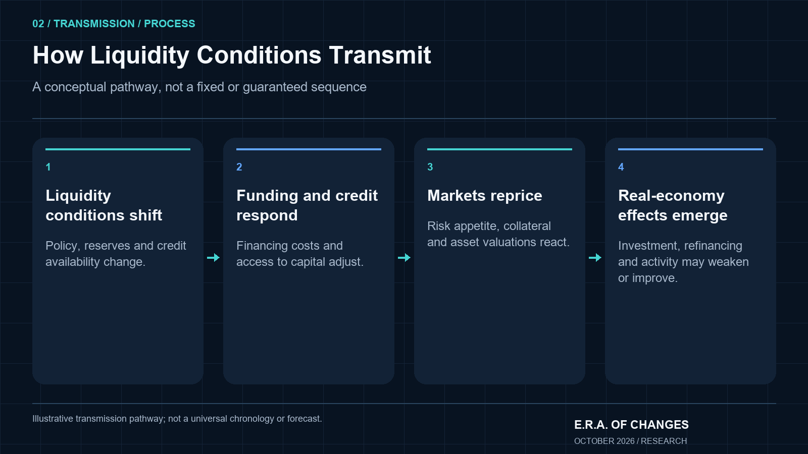
Across the cycles E.R.A. OF CHANGES has studied, a broad pattern tends to recur: central banks and private credit become more supportive → risk appetite and asset prices respond → the expansion produces inflation or excess that triggers policy response → liquidity contracts through rate hikes or QT → weak borrowers struggle → financial stress builds → policy responds with easing → the cycle restarts.

What is important about this sequence for investors is that the financial-market cycle often leads the economic cycle. Liquidity can improve, and risk assets can begin recovering, before GDP has bottomed, before unemployment has peaked, before official recession declarations. Likewise, liquidity can begin tightening while growth still looks strong, which is precisely why 2022’s rate shock hit equity and bond markets so early relative to when the economic slowdown became visible in official data. Financial markets price the direction of liquidity change, not just its current level. This is a core reason why E.R.A. OF CHANGES focuses on identifying changes in the liquidity regime rather than simply observing that current conditions are easy or tight.

Liquidity vs. Solvency

This is a distinction that matters enormously during financial stress, and I want to address it directly because it is frequently conflated.

A liquidity problem occurs when a borrower has genuine assets and underlying value but temporarily cannot access cash (for example, when a bank faces a sudden withdrawal shock but holds performing loans on its balance sheet). Central banks can address this through emergency lending facilities. A solvency problem occurs when a borrower’s assets or cash flow are genuinely insufficient to cover their obligations (for example, when a commercial real-estate property owner cannot generate the debt-service coverage ratio required to refinance, regardless of how much liquidity the Fed provides).

Liquidity support can buy time. It cannot make fundamentally unpayable debt disappear. This is one of the most important limiting principles of any liquidity-based framework: knowing that the Fed will provide emergency liquidity does not resolve the underlying credit quality of borrowers facing the $875 billion in commercial real estate debt maturities in 2026 alone, when refinancing conditions have deteriorated relative to the original loan underwriting. For the full analysis of how that refinancing dynamic creates systemic risk beyond what monetary liquidity can resolve, see Global Debt Risks 2026.

When Liquidity Problems Become Solvency Problems

The progression is worth understanding because it describes how financial stress can accelerate nonlinearly. Funding becomes expensive → refinancing fails → assets are sold to raise cash → prices fall → collateral values decline → losses increase → what began as a liquidity problem becomes a solvency problem for weaker balance sheets.

March 2020 demonstrated this chain in compressed form: within approximately ten days of the initial COVID shock, what began as a liquidity panic (with Treasury markets seizing and money-market funds approaching redemption gates) was heading toward broader solvency stress for airlines, hotels, and other businesses with fixed costs and suddenly zero revenue. The Federal Reserve’s intervention on March 23, 2020, with unlimited QE and a slate of credit facilities, arrested the chain at the liquidity stage before it fully transitioned to mass solvency stress. The speed and scale of that response was without historical precedent. It is also the reason that liquidity analysis must always include an assessment of the policy-response function: how quickly and effectively can central banks intervene if the transmission chain begins to accelerate?

How E.R.A. OF CHANGES Confirms a Liquidity Signal

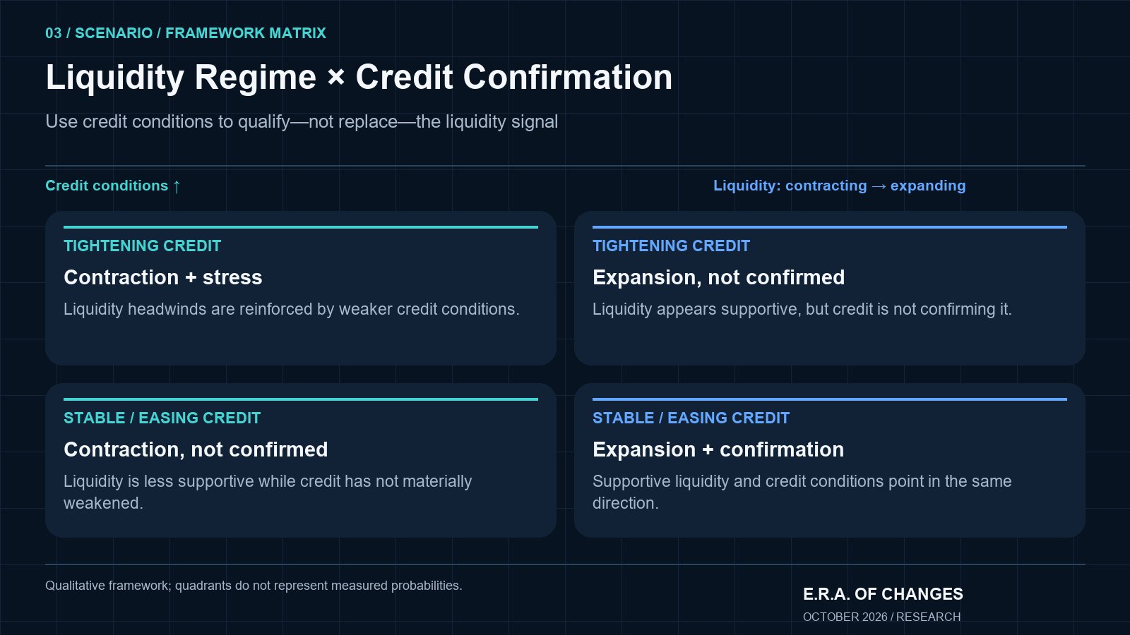
This is important because otherwise liquidity becomes a one-factor model, which it is not designed to be.

E.R.A. OF CHANGES looks for confirmation through credit markets first: are high-yield spreads widening or narrowing? A liquidity contraction that is not yet confirmed by spread widening is a different signal from one where credit markets are deteriorating simultaneously. Then bond volatility: is MOVE rising alongside the liquidity change, or is it stable? Then market breadth: is the liquidity regime supporting the broad market or only a narrow set of mega-cap names? Then funding markets: are repo and cross-currency markets stable or showing unusual pressure? Then, for crypto-oriented analysis, the internal structure of the asset (ETF flows, CME open interest positioning, and on-chain long-term holder behavior) to assess whether the global liquidity signal is being confirmed or overridden by crypto-specific dynamics.

Liquidity provides the regime signal. The other markets help confirm whether that regime is transmitting through the financial system the way history suggests it should.

Common Mistakes When Reading Global Liquidity

Looking only at the Fed balance sheet. This misses the RRP, the TGA, bank reserves, private credit, ECB and BOJ dynamics, and cross-border dollar funding. The Fed’s balance sheet is one input into a seven-variable system.

Treating falling ON RRP usage as automatically bullish. It changes where counterparties hold cash, but the destination matters. Treasury-bill purchases, deposits, and other uses have different implications; a fall in usage does not automatically translate into buying of risk assets. Source.

Treating M2 as the entire liquidity system. M2 is an important domestic measure but misses cross-border dollar conditions, central-bank operations at the institutional level, and private credit dynamics in markets outside M2’s definition.

Ignoring Treasury issuance. When the government issues large volumes of new Treasury securities, it competes for reserves, can crowd out private credit, and can put upward pressure on yields even when the Fed appears accommodative. Fiscal financing is an integral part of the liquidity picture.

Ignoring currency translation. When global central-bank balance sheets are aggregated in U.S. dollar terms, exchange-rate movements can produce apparent expansions or contractions that are purely an FX translation effect rather than a genuine change in liquidity supply. E.R.A. OF CHANGES accounts for this when comparing cross-border balance-sheet trajectories.

Assuming Bitcoin is a mechanical liquidity proxy. Bitcoin has shown high sensitivity to global monetary conditions on a medium-term basis, but it also has independent drivers (ETF flows, regulatory events, network dynamics, and crypto-specific leverage cycles) that can override the macro signal for extended periods.

E.R.A. OF CHANGES Analyst’s Perspective

As of early October 2026, my liquidity assessment is mixed. The Fed had ended securities runoff effective December 1, 2025; consolidated assets were approximately $6.748 trillion on September 23, 2026. Reserve balances averaged approximately $2.93 trillion in the week ended September 23. ON RRP usage was low, but that does not mean the facility was unavailable or that funding stress was inevitable. The composition and distribution of these liabilities matter alongside the asset total. Source. Source 2. Source 3.

On the global side, I compare the major central banks using consistent reporting dates and currency assumptions. BOJ assets of approximately ¥639.6 trillion on June 30, 2026 illustrate its large balance sheet, but do not by themselves establish a historical ranking of policy aggressiveness. Changes in Japanese funding conditions and leveraged currency positions can affect global markets; their scale and timing depend on positioning and the policy response, not on a balance-sheet-to-GDP ratio alone. Source.

I want to be direct: our current liquidity reading is late-cycle mixed rather than clearly supportive or clearly contractionary. The regime is not the expansionary phase of 2020–2021. It is also not the aggressive tightening of 2022. Investors who treat it as either are likely to make positioning errors.

How E.R.A. OF CHANGES Uses Global Liquidity in Its Research Process

Our Forecasting Methodology describes a layered analytical sequence: data signal → historical analogue → liquidity check → market confirmation → instrument analysis → invalidation criteria. Liquidity sits as a central confirmation layer rather than a standalone forecast input. It is not the first question E.R.A. OF CHANGES asks (that is usually the macroeconomic data signal), but it is an early filter on whether conditions are structurally supportive or restrictive for the thesis being formed.

A thesis that depends on risk appetite remaining elevated should be tested against the liquidity regime. If that thesis survives a scenario where liquidity is flat or modestly tightening, it is a stronger thesis than one that only works in an expansionary environment. Conversely, a bearish thesis should be tested against the possibility that fiscal support or central-bank easing provides a liquidity tailwind that delays the transmission of financial stress into equity markets. These invalidation conditions are part of every substantive E.R.A. OF CHANGES research piece, not afterthoughts.

Global Liquidity and Era CrisisMeter

Liquidity conditions are one of the primary dimensions of systemic risk that Era CrisisMeter evaluates, alongside credit conditions, monetary policy trajectory, capital flows, and geopolitical-financial transmission. Understanding global liquidity on its own gives you one layer of the picture. CrisisMeter helps place that layer inside a broader risk framework that accounts for how liquidity interacts with credit stress, funding-market behavior, and systemic risk across multiple dimensions.

The relationship is intended to be sequential rather than redundant: understand the individual liquidity components, then use Era CrisisMeter to assess whether those conditions are translating into broader systemic stress or remaining contained.

Global Liquidity and the Era Global Risk Index

The Era Global Risk Index (updated daily from 24 structural indicators) extends the analysis further. Where global liquidity analysis answers the question of how supportive or restrictive financial conditions are, and Era CrisisMeter answers how severe current systemic stress is, the Era Global Risk Index integrates those signals with macro, geopolitical, and systemic risk dimensions into the broadest composite view E.R.A. OF CHANGES produces. For readers who want to track how the overall risk environment (including dimensions beyond the monetary and credit channels) is evolving, the Era Global Risk Index is the relevant product.

What Global Liquidity Cannot Tell You

It cannot reliably predict exact market tops or bottoms. It cannot forecast every political shock. It cannot provide guaranteed correlations or fixed time lags between global M2 and Bitcoin price; the relationship varies with the sample and institutional environment. It cannot guarantee that monetary easing will reach the real economy if private credit demand is weak. And it cannot determine when a liquidity problem becomes a solvency problem: that depends on the credit quality of specific borrowers, not the aggregate money supply.

Its primary value is identifying whether the financial environment is becoming more supportive or more restrictive for leverage, credit, risk appetite, and the financial conditions under which assets are priced. That is a meaningful analytical tool. It is not an oracle.

A 10-Minute Weekly Global Liquidity Check

For readers who want a practical monitoring routine, the sequence I use starts with the Fed’s weekly H.4.1 release for balance-sheet direction, bank reserves, and the RRP balance. Then Treasury’s daily TGA balance to see whether fiscal cash management is adding or withdrawing liquidity. Then monthly U.S. M2 and, where available, ECB and BOJ broad-money data for the broader monetary picture. Then FRED’s bank-lending surveys when the quarterly SLOOS is released, to assess whether private credit conditions are tightening or easing. Then cross-currency basis markets for any signs of offshore dollar stress, typically revealed in Bloomberg or BIS data on the EUR/USD and JPY/USD basis.

Then the confirmation layer: high-yield spreads and MOVE, which tell you whether the liquidity signal is transmitting into credit and bond-market conditions. And for crypto-specific analysis, U.S. spot Bitcoin ETF flow data, which has become one of the most important real-time indicators of whether institutional capital is entering or leaving the digital asset space.

Compare the aggregate picture against Era CrisisMeter and Our Financial Markets research for how these signals are being integrated into our current systemic-risk assessment.

Three Global Liquidity Regimes

Regime 1: Liquidity Expansion: Major central-bank balance sheets expanding or stabilizing after prior contraction, private credit improving, funding conditions easy, broad money supportive. In this environment, greater risk tolerance and multiple expansion are common tendencies; high-beta assets including crypto often benefit from the combination of easier leverage and rising risk appetite. 2020–2021 was the clearest modern example.

Regime 2: Liquidity Transition: Central banks restrictive but RRP or TGA dynamics partially offsetting conditions, mixed private credit, narrow equity leadership. High dispersion between sectors and asset classes is characteristic; correlations break down. 2023–2024 was a transition regime where aggressive Fed tightening coexisted with surprising equity resilience, precisely because fiscal flows and RRP drawdown were providing an offsetting liquidity buffer.

Regime 3: Liquidity Contraction / Stress: Reserves falling materially, private credit tightening, dollar funding stress appearing in cross-currency markets, spreads widening. Deleveraging, multiple compression, and higher recession and systemic risk are the characteristic tendencies.

Frequently Asked Questions

What is global liquidity?

Global liquidity refers to the availability of money, credit, and financing capacity across the financial system to support economic activity, asset purchases, leverage, and cross-border capital flows. It includes official liquidity created by central banks through balance-sheet operations and private liquidity created through commercial bank lending, capital markets, and cross-border financing. There is no single perfect measure of it. E.R.A. OF CHANGES evaluates seven components together: major central-bank balance sheets, bank reserves, the Fed’s reverse repo facility, Treasury cash management, M2 and broad money, private credit conditions, and cross-border dollar funding.

Why is global liquidity important for investors?

Liquidity affects the cost of leverage, the availability of capital to new buyers, the discount rates applied to future earnings, and aggregate risk appetite. When liquidity is expanding, investors accept higher valuation multiples and greater risk; when it is contracting, multiples compress and leverage is reduced. Understanding the liquidity regime helps investors assess whether market conditions are structurally supportive or restrictive, even before earnings or economic data fully reflect the change.

How is global liquidity measured?

No single measure captures global liquidity accurately. We compare major central-bank balance sheets, reserve balances, ON RRP usage, Treasury cash management, national broad-money measures, private credit conditions, and cross-border dollar funding. Dates and definitions must be consistent: a weekly reserve average is not a Wednesday observation, and a currency-converted global sum is not a single official statistic. Source. Source 2.

Does M2 measure global liquidity?

M2 is one component of our framework, not a complete measure of global liquidity. U.S. seasonally adjusted M2 was $23.3428 trillion in August 2026 in the September 22 H.6 release. It excludes many cross-border funding channels and does not measure all private credit or central-bank operations. National monetary aggregates cannot be added into an official global total without specifying their definitions and currency-conversion method. Source.

How does the Federal Reserve balance sheet affect markets?

The Fed’s balance sheet affects markets primarily through its impact on bank reserves, funding conditions, and the cost of leverage. When the balance sheet expands through quantitative easing, reserves flow into the banking system and funding conditions typically ease. When it contracts through QT, reserves fall and funding can become more expensive for marginal participants. But the relationship is not direct: the net effect depends on where reserves flow, what the Treasury General Account is doing simultaneously, and whether private credit conditions are amplifying or offsetting the central-bank signal. The Fed’s balance sheet ended QT in December 2025 and has grown modestly since, but this does not by itself constitute a significant liquidity expansion.

What is the reverse repo facility and why does it matter?

ON RRP lets eligible counterparties place cash with the Fed against securities overnight and helps implement the policy-rate floor. Usage reached roughly $2.5 trillion in 2022 and subsequently fell to very low levels. A decline can offset some reserve drainage, depending on where the cash moves. It is not an emergency lending facility, and low usage does not prove that the financial system has lost its ability to absorb shocks. Source.

What is the Treasury General Account and how does it affect liquidity?

The TGA is Treasury’s operating account at the Fed. Spending generally adds reserves and bank deposits; rebuilding cash can absorb them. The net effect depends on how debt buyers finance their purchases and on other changes in Fed liabilities, including ON RRP. For that reason, Treasury cash balances should be interpreted alongside issuance, spending, and reserve data rather than as a standalone risk-asset signal. Source. Source 2. Source 3.

How does global liquidity affect Bitcoin?

Bitcoin has shown significant medium-term sensitivity to global monetary conditions. The relationship between global M2 and Bitcoin varies across samples and time windows, and correlation does not establish how much M2 explains Bitcoin’s price moves. It is not mechanical: timing varies, and institutional ETF flows or other factors can outweigh the macro signal for a time. E.R.A. OF CHANGES treats global liquidity as a regime indicator for Bitcoin (explaining the broad cycle context) rather than a pricing model.

What happens when global liquidity contracts?

Liquidity contraction typically produces higher funding costs, reduced leverage capacity, tighter credit conditions, wider credit spreads, and greater vulnerability for weak balance sheets. High-beta assets including crypto are often early to feel the pressure. The most serious risk is when liquidity contraction combines with credit deterioration and funding-market stress, producing the self-reinforcing deleveraging dynamic that characterizes financial stress episodes.

Does more liquidity always make markets rise?

No. Markets can fall in an expanding liquidity environment if earnings collapse, a geopolitical shock forces deleveraging, a banking crisis impairs credit transmission, or extreme valuations mean the liquidity tailwind is insufficient to offset deteriorating fundamentals. Conversely, markets can remain resilient in a contracting environment if fiscal support is offsetting monetary tightening, corporate buybacks and passive flows provide mechanical demand, or earnings growth is genuinely strong enough to compensate for multiple compression. Liquidity changes probabilities; it does not dictate every short-term market move.

How does E.R.A. OF CHANGES use global liquidity in its research?

E.R.A. OF CHANGES uses global liquidity as a central confirmation layer in its Forecasting Methodology: a filter on whether conditions are structurally supportive or restrictive for the macro thesis being formed. Liquidity is not the first question E.R.A. OF CHANGES asks (that is typically the macroeconomic data signal), but it is an early and important input before E.R.A. OF CHANGES moves to credit-market confirmation, funding-market behavior, and cross-asset analysis. our CrisisMeter and Global Risk Index then place the liquidity reading inside the broader systemic-risk framework.

About E.R.A. OF CHANGES

E.R.A. OF CHANGES publishes macroeconomic research, financial-market analysis, and geopolitical risk assessments. Our work combines quantitative indicators with analyst judgment in proprietary research frameworks. These frameworks are tools for interpreting risk, not guarantees of future performance or independently calibrated event probabilities. Readers can explore our methodology, forecast archive, and research catalogue on the website.

The content published by E.R.A. OF CHANGES is for informational and educational purposes only and does not constitute financial, investment, legal, or tax advice. All views expressed are the personal analytical perspective of the author. Past forecast accuracy does not guarantee future results. Readers should conduct their own research and consult a qualified financial professional before making any investment decisions.

Sources

Central-Bank Balance Sheets and Reserves - Federal Reserve H.4.1, September 24, 2026 - Federal Reserve: Securities Runoff Ends December 1, 2025 - Bank of Japan Accounts, June 30, 2026

Money and Funding - Federal Reserve H.6 Money Stock Measures, September 22, 2026 - New York Fed: Overnight Reverse Repo Facility FAQ - U.S. Treasury: Daily Treasury Statement

Market and Fiscal Context - FRED: ICE BofA U.S. High Yield Index Option-Adjusted Spread - Nasdaq Index Performance: December 2022 - U.S. Treasury: Fiscal Year 2022 Budget Results - Bitcoin.org: Bitcoin Halving

Internal E.R.A. OF CHANGES Research - Era CrisisMeter Explained - Era Global Risk Index - Era Forecasting Methodology - What Is M2 Money Supply? - How Interest Rate Hikes Affect Markets - Bitcoin Cycles Explained - Bitcoin ETF Adoption Report - Global Debt Risks 2026 - Yield Curve Explained - Financial Stress Indicators Explained - Global Recession Probability Report - Gold Market Outlook 2026 - Global Inflation Drivers 2026